(This is a blogpost version of a talk I gave at MLConf SF 11/14/2014. See below for original video and slides)
There are many good textbooks and courses where you can be introduced to machine learning and maybe even learn some of the most intricate details about a particular approach or algorithm (See my answer on Quora on what are good resources for this). While understanding that theory is a very important base and starting point, there are many other practical issues related to building real-life ML systems that you don’t usually hear about. In this post I will share some of the most important lessons learned in years of building large-scale ML solutions that power products such as Netflix and scale to millions of users across many countries.
And just in case it doesn’t come across clearly enough, let me insist on this once again: it does pay off to be knowledgeable and have deep understanding of the techniques and theory behind classic and modern machine learning approaches. Understanding how Logistic Regression works or the difference between Factorization Machines and Tensor Factorization, for example, is a necessary starting point. However, this in itself might not be enough unless you couple it with the real-life experience of how these models interact with systems, data, and users in order to obtain a really valuable impact. The next ten lessons are my attempt at trying to capture some of that practical knowledge.
1. More Data vs. and Better Models
A lot has been written about whether the key to better results lays in improving your algorithms or simply on throwing more data at your problem (see my post from 2012 discussing this same topic, for example).
In the context of the Netflix Prize, Anand Rajaraman took an early stand on the issue by claiming that “more data usually beats better algorithms”. In his post he explained how some of his students had improved some of the existing results on the Netflix ratings dataset by adding metadata from IMDB.
 |
|---|
| Fig 1. More data usually beats better algorithms |
Although many teams in the competition tried to follow that lead and add extra features to improve results, there was little progress in that direction. As a matter of fact, just a year later some of the leaders of what would become the runner up team published a paper in which they showed that adding metadata had very little impact in improving the prediction accuracy of a well-tuned algorithm. Take this as a first example of why adding more data is not always the solution.
|  |
|—|
| Fig 2. Even a Few Ratings Are More Valuable than Metadata |
|
|—|
| Fig 2. Even a Few Ratings Are More Valuable than Metadata |
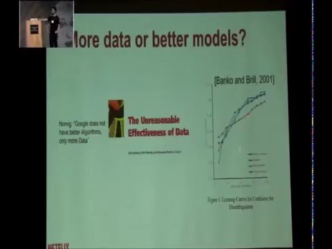
Of course, there are different ways to “add more data”. In the example above we were adding data by increasing the number and types of features, therefore increasing the dimensionality of our problem space. We can think about adding data in a completely different way by fixing the space dimensionality and simply throwing more training examples at it. Banko and Brill showed in 2001 that in some cases very different algorithms responded equally well by improving to more training data (see figure below)
 |
|---|
| Fig 3. Banko and Brill’s “famous” model performance curves |
Google’s Research Director and renowned AI figure Peter Norvig is quoted as saying that “Google does not have better algorithms, just more data”. In fact, Norvig is one of the co-authors of “The Unreasonable Effectiveness of Data where in a similar problem to the one in Banko and Brill (language understanding) they also show how important it is to have “more data”.
 |
|---|
| Fig 4. The Unreasonable Effectiveness of Data |
So, is it true that more data in the form of more training examples will always help? Well, not really. The problems above are complex models with a huge number of features which lead to situations of “high variance“. But, in many other cases this might not be true. See below for example a real-case scenario of an algorithm in production at Netflix. In this case, adding more than 2 million training examples has very little to no effect.
 |
|---|
| Fig 5. Testing Accuracy of a real-life production model |
So, this leads to our first lesson learned, which in fact will expand over several of the following ones: it is not about more data versus better algorithms. That is a false dichotomy. Sometimes you need more data, and sometimes you don’t. Sometimes you might need to improve your algorithm and in others it will make no difference. Focusing exclusively on one or the other will lead to far from optimal results.
2. You might not need all your “Big Data”
This second lesson is in fact a corollary of the previous one, but I feel it is worth to mention explicitly on its own. It seems like nowadays everyone needs to make use of all their “Big Data”. Big Data is so hyped that it seems like if you are not using huge quantities of data you must be doing something wrong. The truth though, as discussed in lesson 1, is that there are many problems for which you might be able to get similar results by using much less data than the one you have available.
Think for example of the Netflix Prize where you had 0.5 Million users in the dataset. In the most favored approach, the data was used to compute a Matrix of 50 factors. Would the result change much if instead of the 0.5 M users you used, say 50 Million? Probably not.
A related, and important, question is how do you determine what subset of your data to use. A good initial approach would be to random sample your original data to obtain as many samples you need for your model training. That might not be good enough though. Staying with the Netflix Prize example, users might be very different and not homogeneously distributed in our original population. New users, for example, will have much fewer ratings and increase sparsity in the dataset. On the other hand, they might have a different behavior from more tenured users and we might want to make our model capture it. The solution is to use some form of stratified sampling. Setting up a good stratified sampling scheme is not easy since it requires us to define the different strata, and decide what is the right combination of samples for the model to learn. However, as surprising as it might sound, a well-defined stratified sampled subset might accomplish even better results than the original complete dataset.
Just to be clear, I am not saying that having lots of data is a bad thing, of course it is not. The more data you have, the more choices you will be able to make on how to use it. All I am saying is that focusing on the “size” of your data versus the quality of the information in the data is a mistake. Garner the ability to use as much data as you can in your systems and then use only as much as you need to solve your problems.
3. The fact that a more complex Model does not improve things does not mean you don’t need one
Imagine the following scenario: You have a linear model and for some time you have been selecting and optimizing features for that model. One day you decide to try a more complex (e.g. non-linear) model</span> with the same features you have been engineering. Most likely, you will not see any improvement.
After that failure, you change your strategy and try to do the opposite: You keep the old model, but
add expressive features that try to capture more complex interactions. Most likely the result will be the same and you will again see little to no improvements.
So, what is going on? The issue here is that simply put more complex features require a more complex model, and vice versa, a more complex model may require more complex features before showing any significant improvement.
So, the lesson learned is that you must improve both your model and your feature set in parallel. Doing only one of them at a time might lead to wrong conclusions. </div>
4. Be thoughtful about how you define your training/testing data sets
If you are training a simple binary classifier, one of the first tasks to do is to define your positive and negative examples. Defining positive and negative labels for samples though may not be such a trivial task. Think about a use case where you need to define a classifier to distinguish between shows that users watch (positives) and do not watch (negatives). In that context, would the following be positives or negatives?
- User watches a movie to completion and rates it 1 star
- User watches the same movie again (maybe because she can’t find anything else)
- User abandons movie after 5 minutes, or 15 minutes… or 1 hour
- User abandons TV show after 2 episodes, or 10 episode… or 1 season
- User adds something to her list but never watches it
As you can see, determining whether a given example is a positive or a negative is not so easy.
Besides paying attention to your positive and negative definition, there are many other things you need to make sure to get right when defining your training and testing datasets. One such issue is what we call Time Travelling. Time traveling is defined as usage of features that originated after the event you are trying to predict. E.g. Your rating a movie is a pretty good prediction of you watching that movie, especially because most ratings happen AFTER you watch the movie.
In simple cases as the example above this effect might seem obvious. However, things can get very tricky when you have many features that come from different sources and pipelines and relate to each other in non-obvious ways. Time traveling has the effect of increasing model performance beyond what would seem reasonable. That is why whenever you see an offline experiment with huge wins, the first question you might want to ask yourself is: “Am I time traveling?”. And, remember, Time Traveling and positive/negative selection are just two examples of issues you might encounter when defining your training and testing datasets. Just make sure you are thoughtful about how you define all the details of your datasets.
5. Learn to deal with (the curse of) the Presentation Bias
 |
|---|
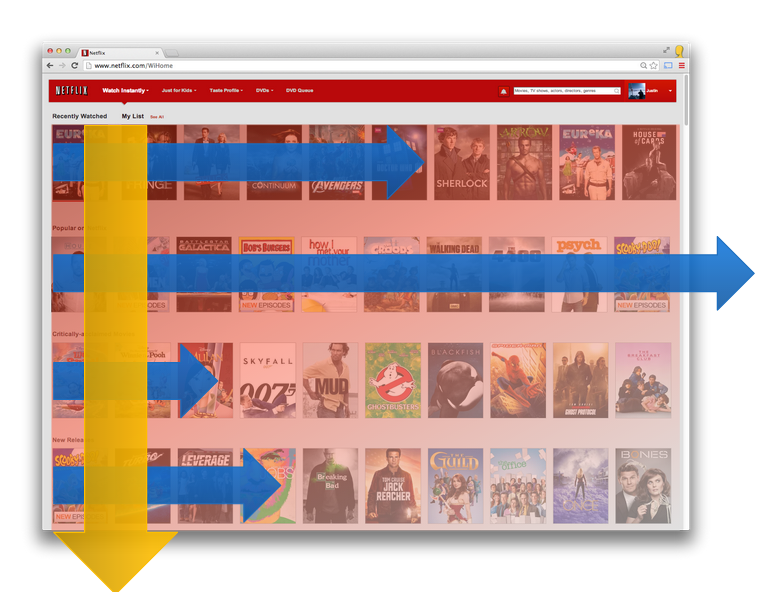
| Fig 6. Example of an Attention Model on a page |
Let’s face it, users can only click and act on whatever your algorithm (and other parts of your system) has decided to show them. Of course, what your algorithm decided to show is what it predicted was good for the user. Let’s suppose that a new user comes in and we decide to show the user only popular items. The fact that a week later the user has only consumed popular items does not mean that’s what the user like. That’s the *only* thing she had a chance to consume!
As many (including myself) have mentioned in the past, is important to take that into account in your algorithms and try to somehow break this “Curse of the Presentation Bias”. Most approaches to addressing this issue are based on the idea that you should “punish” items that were showed to the user but not “clicked on”. One way to do so is by implementing some presentation discounting mechanism (see this KDD 2014 paper by the LinkedIn folks).
Another way to address the issue is to use viewed but not clicked items as negatives in your training process. This, in principle, makes sense: if a user searched for a query and ended up clicking in result number three it means the first two results were bad and should be treated as negatives… or not? The problem with this is that although the first two items were likely worse than the third one (at least in that particular context), this does not mean they were any worse than item in position 4, let alone item in position 5000, which your original model decided was no good at all. Yes, you want to remove the presentation bias, but not all of it since it responds to some hopefully well-informed decisions your model took in the first place.
So, what can we do? First thing that comes to mind is to introduce some sort of randomization in the original results. This randomization should allow to collect unbiased user feedback so as to whether those items are good or not (see some of the early publications by Thorsten Joachims such as this one or take a look at the idea of result dithering proposed by Ted Dunning).
Another better approach is to develop some sort of “attention model” of the user. In this case both clicked and non-clicked items will be weighted by the probability that the user noticed them in the first place depending on their location on the page (see some of the recent work by Dmitry Lagun for interesting ideas on this area.
Finally, yet another and well established way to address presentation bias is by using some sort of explore/exploit approach, in particular multi-armed bandits. By using a method such as Thompson Sampling, you can introduce some form of “randomization” on the items that you are still not sure about, while still exploiting as much as you can from what you already know for sure (see Deepak Argawal’s Explore/Exploit approach to recommendations or one of the many publications by Thorsten Joashims for more details on this).
6. The UI is the only communication channel between the Algorithm and what matters most: the Users
 |
|---|
| Fig 7. The UI is the algorithm’s connection point with the user |
From the discussion in the previous lesson it should be clear by now how important it is to think about the presentation layer and the user interface in our machine learning algorithmic design. On the one hand, the UI generates all the user feedback that we will use as input to our algorithms. On the other hand, the UI is the only place where our algorithms will be shown. It doesn’t matter how smart our ML algorithm is. If the UI hides its results or does not give the user the ability to give some form of feedback, all our efforts on the modeling side will have been in vain.
Also, it is important to understand that a change in the user interface might require a change in the algorithms and vice versa. Just as we learned before that there is an intimate connection between features and models, there is also another to be aware of between the algorithms and the presentation layer.
7. Data and Models are great. You know what is even better? The right evaluation approach.
 |
|---|
| Fig 8. Offline/Online Innovation Approach |
This is probably one of the most important of the lessons in this post. Actually, as I write this I feel that it is a bit unfortunate that this lesson might seem as “just another lesson” hidden in position 7. This should be a good place to stress that these lessons in this post are not sorted from more to less important, they are just grouped in topics or themes.
So, yes, as important as all the other discussions about data, models, and infrastructure may be, they are all rather useless if you don’t have the right evaluation approach in place. If you don’t know how to measure an improvement you might be endlessly spinning your wheels without really getting anywhere. Some of the biggest gains I have seen in practice have indeed come from tuning the metrics to which models were being optimized.
Ok, then what is the “right evaluation approach”? Figure 8 illustrates an offline/online approach to innovation that should be a good starting point. Whatever the final goal of your machine learning algorithm is in your product you should think of driving your innovation in two distinct ways: offline and online.
 |
|---|
| Fig 9. Offline Evaluation |
First, you should generate datasets that allow to try different models and features in an offline fashion by following a traditional ML experimentation approach (see Figure 9): You train your model to a training seat, you probably optimize some (hyper)parameters to a validation set, and finally measure some evaluation metrics on a test set. The evaluation metrics in our context are likely to be IR metrics such as precision and recall, ROC curves, or ranking metrics such as NDCG, MRR, or FPC (Fraction of Concordant Pairs). Note though that the selection of the metric itself has its consequences. Take a look at Figure 10 for an example of how the different ranking metrics weight different ranks being evaluated. In that sense, metrics such as MRR or (especially) NDCG will give much more importance to the head of the ranking, while FPC will be weighting more on the middle of the ranks. The key here is that depending on your application you should choose the right metric.
 |
|---|
| Fig. 10. Importance given to different ranks by typical ranking metrics |
Offline experimentation is great because once you have the right data and the right metric it is fairly cheap to run many experiments with very few resources. Unfortunately, a successful offline experiment can only be generally used as an indication of a promising approach worth testing online. While most companies are investing in finding better correlation between offline and online results, this is still, generally speaking, an unsolved issue that deserves more research (see this KDD 2013 paper, for example).
In online experimentation the most usual approach is to do A/B testing (other approaches such as Multiarmed Bandit Testing or Interleaved Testing are becoming more popular recently but are beyond the scope of this post). The goal of an A/B test is to measure difference in metrics across statistically identical populations that each experience a different algorithm. As with the offline evaluation process, and perhaps even more here, it is very important to choose the appropriate evaluation metric to make sure that most if not all decisions on the product are data driven.
Most people will have a number of different metrics they are tracking in any AB test, but it is important to clearly identify the so-called Overall Evaluation Criteria (OEC). This should be the ultimate metric used for product decisions. In order to avoid noise and make sure the OEC maps well to business success it is better to use a long-term metric (e.g. customer retention). Of course, the issue with that is that you need time, and therefore resources, to evaluate a long-term metric. That is why it is very useful to have short-term metrics that can be used as initial early reads on the tests in order to narrow down worthwhile hypothesis that need to wait until the OEC read is complete.
If you want more details on the online experimentation piece there are many good reads, starting with the many good articles by Bing’s Ronny Kohavi (see this, for example).
8. Distributing algorithms? Yes, but at what level?
There always comes a time in the life of a Machine Learning practitioner when you feel the need to distribute your algorithm. Distributing algorithms that require of many resources is a natural thing to do. The issue to consider is at what *level* does it make sense to distribute.
We distinguish three levels of distribution:
- Level 1. For each independent subset of the overall data
- Level 2. For every combination of the hyperparameters
- Level 3. For all partitions in each training dataset
In the first level we may have subsets of the overall data for which we need to (or simply can) train an independently optimized model. A typical example of this situation is when we opt for training completely independent ML models for different regions in the world, different kinds of users, or different languages. In this case, all we need to do is to define completely independent training datasets. Training can then be fully distributed requiring no coordination or data communication.
In the second level, we address the issue of how to train several models with different hyperparameter values in order to find the optimal model. Although there are smarter ways to do it, let’s for now think of the worst-case grid search scenario. We can definitely train models with different values of the hyperparameters in a completely distributed fashion, but the process does require coordination. Some central location needs to gather results and decide on the next “step” to take. Level 2 requires data distribution, but not sharing since each node will use a complete replica of the original dataset and the communication will happen at the level of the parameters.
Finally, in level 3 we address the issue of how to distribute or parallelize model training for a single combination of the hyperparameters. This is a hard problem, but there has been a lot of research put into it. There are different solutions with different pros and cons. You can distribute computation over different machines splitting examples or parameter using, for example, ADMM. Recent solutions such as the Parameter Sever promise to offer a generic solution to this problem. Another option is to parallelize on a single multicore machine using algorithms such as Hogwild. Or, you can use the massive array of cores available in GPU cards.
As an example of the different approaches you can take to distribute each of the levels, take a look at what we did in our distribution of Artificial Neural Networks over the AWS cloud (see Figure 11 below for an illustration). For Level 1 distribution, we simply used different machine instances over different AWS regions. For Level 2 we used different machine in the same region and a central node for coordination. We used Condor for cluster coordination (although other options such as StarCluster, Mesos, or even Spark) are possible. Finally, for level 3 optimization, we used highly optimized CUDA code on GPUs.
 |
|---|
| Fig 11. Distributing ANN over the AWS cloud |
9. It pays off to be smart about your Hyperparameters
 |
|---|
| Fig 12. Example of model accuracy vs. regularization lambda |
I should also add that even though in this lesson I have dsf about using a brute-force grid search approach to hyperparameter optimization, there are much better things you can do which are again beyond the scope of this post. If you are not familiar with Bayesian Optimization, start with this paper or take a look at Spearmint or MOE.
10. There are things you can do Offline and there are things you can’t… and there is Nearline for everything in between
 ](/blog/images/MachineLearningArchitecture-v3.jpg) ](/blog/images/MachineLearningArchitecture-v3.jpg) |
|---|
| Fig 13. This three level architecture can be used as a blueprint for machine learning systems that drive customer impact. |
Interestingly, thinking about these three “shades of latency” also helps breaking down traditional machine learning algorithms into different components that can be executed in different layers. Take matrix factorization as an example. As illustrated in Figure 14, you can decide to do the more time-consuming item factor computation in an offline fashion. Once those item factors are computed, you can compute user factors online (e.g. solving a closed-from least squares formulation) in a matter of milliseconds in an online fashion.
 |
|---|
| Fig 14. Decomposing matrix factorization into offline and online computation |
If you are interested in this topic take a look at our original blog post in the Netflix tech blog.
Conclusions
The ten lessons in this post illustrate knowledge gathered from building impactful machine learning and general algorithmic solutions. If I had to summarize them in 4 short take away messages those would probably be:
- Be thoughtful about your data
- Understand dependencies between data and models
- Choose the right metric
- Optimize only what matters
I hope they are useful to other researchers and practicioners. And, would love to hear about similar or different experiences in building real-life machine learning solutions in the comments. Looking forward to the feedback.
Acknowledgments
Most of the above lessons have been learned in close collaboration with my former Algorithms Engineering team at Netflix. In particular I would like to thank Justin Basilico for many fruitful conversations, feedback on the original drafts of the slides, and for providing some of the figures in this post.
